- 社交网络与文本分析课程
5 网络基本拓扑性质
刘跃文 教授、博导西安交通大学 管理学院
联系方式: liuyuewen@xjtu.edu.cn2023年4月16日 版本1.2
1. 网络连通性
- 连通(connected):每对节点之间都存在路径
- 连通片(conneted component):连通的孤立子图(subgraph)
- 不连通(disconneted):由多个连通片组成
- 最大连通片(maximal conneted component):包含顶点数最多的连通片
- 有向图
- 图中任何两个节点都有路径(不考虑沿边的方向前进),则为弱连通图
- 考虑沿着边的方向前进,图中任何两个节点存在有向路径,则为强连通图
import networkx as nx
import matplotlib.pyplot as plt

#networkx自带的“风筝”网络图,命名为G_kite
G_kite=nx.krackhardt_kite_graph()
fig, ax1 = plt.subplots(figsize=(13, 4))#调整画布尺寸
plt.subplot(121)
nx.draw_networkx(G_kite)

#删除5-7节点对应的边,6-7节点对应的边,命名为G_kite_cut
G_kite_cut=nx.krackhardt_kite_graph()
G_kite_cut.remove_edge(5,7)
G_kite_cut.remove_edge(6,7)
plt.subplot(122)
nx.draw_networkx(G_kite_cut)

#判断是否是连通图
print('风筝网络图是否是连通图:',nx.is_connected(G_kite))
print('修剪后的风筝网络图是否是连通图:',nx.is_connected(G_kite_cut))
print('风筝网络图连通片数目:',nx.number_connected_components(G_kite))
print('修剪后的风筝网络图连通片数目:',nx.number_connected_components(G_kite_cut))
print('修剪后的风筝网络图连通片情况为:',list(nx.connected_components(G_kite_cut)))
print('修剪后的风筝网络图最大连通片为:',max(nx.connected_components(G_kite_cut), key=len))
1.1 无向网络中的巨片
- 全世界只要有一个人没朋友或只要有一小群人没有除了这群人之外的朋友,那整个网络不连通(连通性是一个脆弱的性质)
- 但是一个人所处的连通片可以非常大
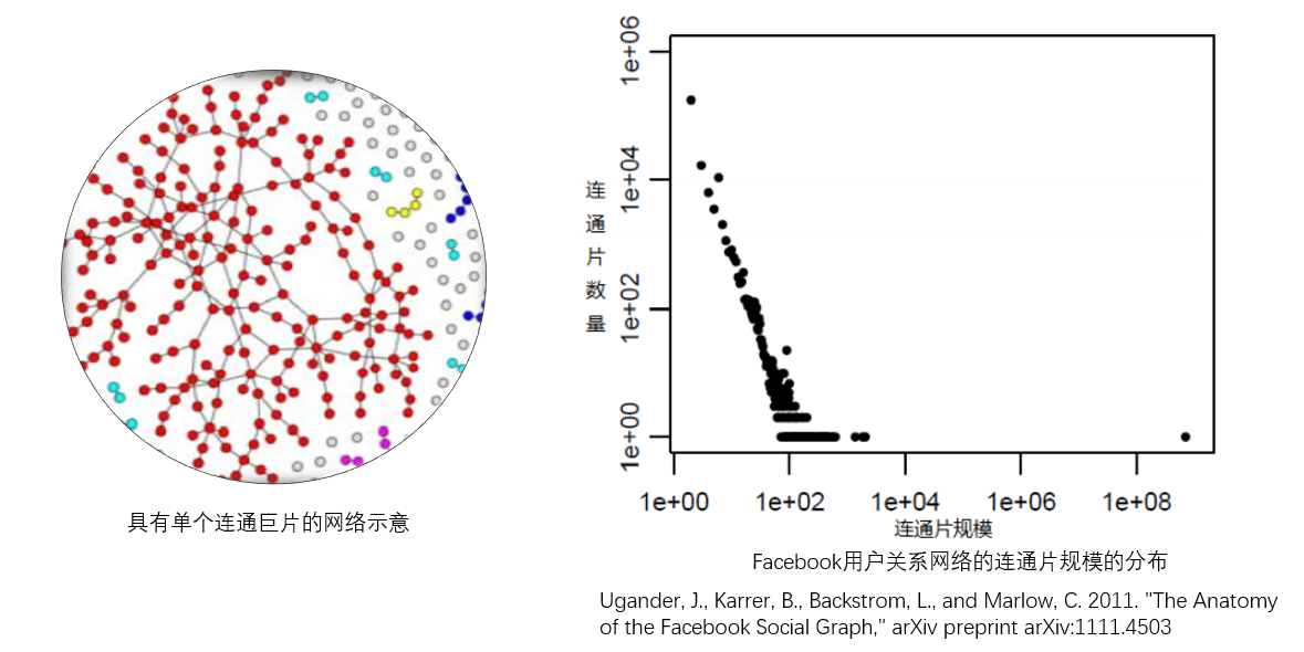
- 巨片(giant component):许多实际的大规模网络都是不连通的,但往往会存在一个特别大的连通片,它包含了整个网络相当比例的节点
- 无向网络的连通巨片的存在唯一性!
- 食堂数据社交网络
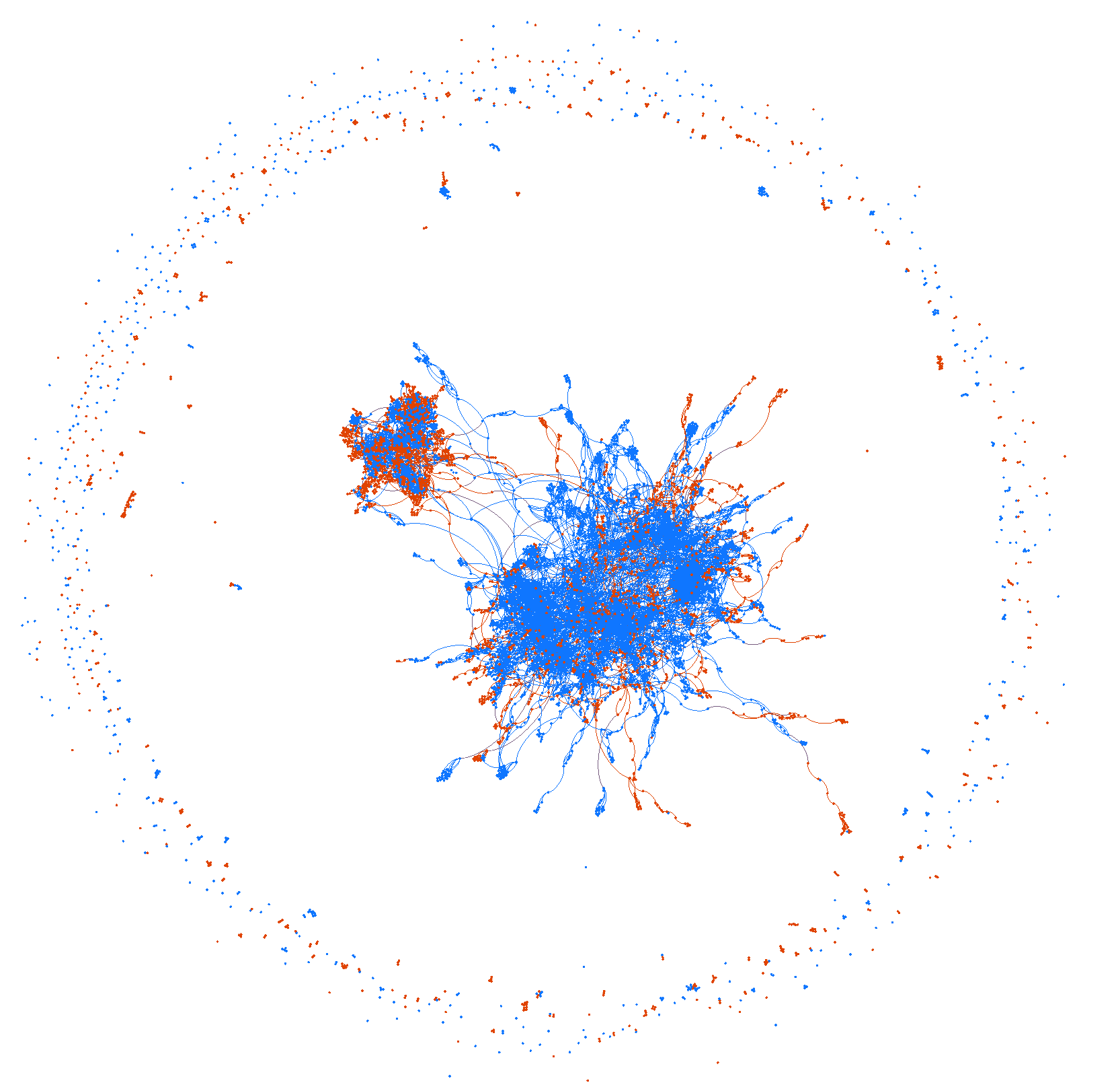
1.2 有向网络中的蝴蝶结结构
- 弱连通巨片(Giant weakly connected component, GWCC):有向网络有一个包含了网络中相当部分节点的很大的弱连通片
- 具有蝴蝶结结构(Bow-tie structure)
- 强连通核 (Strongly connected core, SCC)
- 入部 (IN)
- 出部 (OUT)
- 卷须部 (TENDRILS)


2. 网络稀疏性
2.1 网络密度
- 密度D,density
- 定义:网络中实际存在的边数M与最大可能的边数之比
- $\rho=\frac {M} {\frac{1}{2}N(N-1)}$, M为网络边数,N为网络节点数
- 如果是有向网络,最大可能的边数变为$N(N-1)$
- 含义:网络密度越大,意味着实际存在的边数越多,也意味着网络越稠密;反之,网络越稀疏
- 对网络密度的理解,参考链接:http://olizardo.bol.ucla.edu/classes/soc-111/textbook/_book/6-9-graph-density.html#why-is-density-important
- 密度大的网络更利于信息传播
- 密度大的网络更容易应对网络被破坏(如关键人物的消失)
print('风筝网络图的密度:',nx.density(G_kite))#结果为0.4
2.2 富人俱乐部
富人俱乐部系数:某一类人群形成网络的密度
度数大于k的节点的连接情况
$\text{rich club coefficient}=\frac{M_{>k}}{\frac{1}{2}N_{>k}(N_{>k}-1)}$
分子为度数大于$k$节点网络实际边数,分母为度数大于$k$节点网络可能的最大边数
网络中度值高的节点之间的连接,往往表示出比度值低的节点之间的连接更加紧密的趋势
上述定义在随机网络中也能检测出富人俱乐部现象。Colizza et al. 2006, Nature Physics 提出了标准化富人俱乐部系数。

3. 平均路径长度和直径
3.1 复习概念
- 路径?
- 路径长度?
- 最短路径?
3.2 网络的平均路径长度 L (Avearge path length)
- 定义:网络中任意两个节点之间距离的平均值
- 公式:$L=\frac {1} {\frac{1}{2}N(N-1)}\sum_{i\geq j} {d_{ij}}$
- 可能两个节点之间不存在连通的路径,则这两个节点之间的距离无穷大,导致网络平均路径也是无穷大
- 处理方式1:存在连通路径的节点对之间的距离的平均值 (python networkx计算的)
- 处理方式2:网络中两点之间距离的简谐平均(Harmonic mean):$L=\frac {1} {GE}$,$GE=\frac {1} {\frac{1}{2}N(N-1)}\sum_{i\geq j} \frac{1}{d_{ij}}$
print('风筝网络图的平均最短路径:',round(nx.average_shortest_path_length(G_kite),3))#返回图G所有节点间平均最短路径长度,保留三位小数
print('风筝网络图的直径:',nx.diameter(G_kite))#返回图G的直径(最长最短路径的长度)
# print('风筝网络图的平均最短路径:',round(nx.average_shortest_path_length(G_kite_cut),3))#报错,说明计算的是连通图的最短路径
3.3 六度分隔/六度空间理论/小世界现象 Six degrees of separation
- 六度空间理论的网络演绎版本:“你和任何一个陌生人之间所间隔的人不会超过六个,也就是说,最多通过五个中间人你就能够认识任何一个陌生人。这个理论说明,虽然世界很大,但其实也很小。小到最多通过5个人你就能认识任何一个陌生人。”

- 文献回顾与历史:
- 1909,Guglielmo Marconi根据他在无线电研究工作中提出的猜想(详见他1909年发表的诺贝尔演讲辞)诺贝尔演讲辞链接:https://www.nobelprize.org/nobel_prizes/physics/laureates/1909/marconi-lecture.pdf
- 1929,启发了匈牙利作家Frigyes Karinthy写成了一个人至多通过五个人寻找另外一个人的挑战的故事《链》(Chains)。
- 1967,哈佛大学社会心理学家Stanley Milgram将一套连锁信件随机发送给居住在内布拉斯加州奥马哈的160个人,信中放了一个波士顿股票经纪人的名字,信中要求每个收信人将这套信寄给自己认为比较接近股票经纪人的朋友。朋友收信后照此办理。“最终,大部分信件经过五、六个步骤后都抵达了该股票经纪人”。【樊瑛教授 复杂网络分析课件】
- 文献参考:Miltram, S. Psychol. Today 1, 61-67 (1967)

真实的情况:
- “首次连锁信件实验(50人),只有三封信送到了目的地。在随后两次连锁信实验,因完成连锁的比例太低,实验结果未被发表。”
“虽然饱受议论,米尔格伦带来不少新奇的发现。经过多次改良实验,米尔格伦发现信件或包裹在人们心目中的价值是影响人们决定继续传递它的重要因素。他成功将送达率提升至35%, 以至于后来更上升为97%。”“不仅如此,米尔格伦还发现了漏斗效应, 他发现大部分的传递都是由那些极少数的明星人物完成的。在一个5%的飞行员实验中,他发现2/3成功的传递是由同一些“明星”来完成的。” 【百度百科】
不要人云亦云。大胆假设,小心求证。
Milgram实验:
- 权力服从研究(Milgram experiment,又称Obedience to Authority Study)是一个针对社会心理学非常知名的科学实验。实验的概念最先开始于1963年由耶鲁大学心理学家斯坦利·米尔格拉姆在《变态心理学杂志》(Journal of Abnormal and Social Psychology)里所发表的Behavioral Study of Obedience 一文,稍后也在他于1974年出版的Obedience to Authority: An Experimental View里所讨论。这个实验的目的,是为了测试受测者,在面对权威者下达违背良心的命令时,人性所能发挥的拒绝力量到底有多少。
https://baike.baidu.com/item/%E7%B1%B3%E5%B0%94%E6%A0%BC%E5%85%B0%E5%A7%86/10644763?fr=aladdin
Stanley Milgram与Paul Milgrom


3.4 Facebook的用户之间平均距离
- Facebook计算社会关系的基础是朋友关系。如果A是B的Facebook好友,B又是C的Facebook好友,则可以认为A可以通过B认识C,A与C之间的间隔就是1。
- 2016年利用了 Flajolet-Martin 算法来估算每个人从某个来源能够认识到的新人的数量。最终统计出 Facebook 用户之间的平均间隔区间为 2.7 到 4.7 之间,而中位数为 3.57。
- 2008年平均分离度为5.28, 2011年为4.74,2016年为3.57

- Erdos鄂尔多斯数
- Erdos是20世纪最伟大的天才数学家之一。他的论文涵盖数学各个分支领域,甚至统计、物理等跨学科领域。Erdos发表论文如同开挂,战斗力惊人。据说他每天工作19小时,在古稀之年仍然如此。他毕生发表过的数学论文超过1500篇,在数学史上仅次于神级人物欧拉(Euler)。Erdos广泛的研究兴趣使得他有超好的“人缘”。据不完全统计,他的合作者超过450人,若加上别人所作但曾获他关键性的提示的论文,则总数应有数万篇。
- Erdos数。这个数字的设计原理非常简单:Erdos本人的Erdos数是0;曾与Erdos合作发表过文章的人的Erdos数是1;没有与Erdos合作发表过文章,但与Erdos数为1的人合作过的是2。 https://www.oakland.edu/enp/compute/

- Bacon贝肯数
- 贝肯是好莱坞的一名普通演员,不同于马龙·白兰度这样的大腕,贝肯在好莱坞电影中从来都是以配角的身份出现,他与当时好莱坞的影视明星发生联系所需要的中间人数量即为“贝肯数”。弗吉尼亚大学一个实验室曾为约25万上过银幕的男女演员计算了他们的“平均贝肯数”,研究发现无论是历史上贝肯数最低的演员罗德·斯泰格尔还是一个名不见经传的小演员,他们的贝肯数都在2.6和3之间,并且相差十分微小。http://oracleofbacon.org/
3.5 直径 D(Diameter)
- 定义:网络中任意两个节点之间距离的最大值
- 公式:$D=max {d_{ij}}$
- 实际应用中,指的是任意两个存在有限距离的(i.e.,连通的)节点的距离的最大值
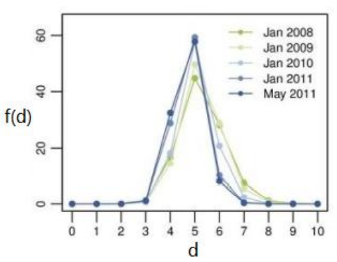
- 网络中绝大部分用户对之间的距离,有效直径的概念(以Facebook为例)
- f(d) 距离为d的连通的节点对的比例
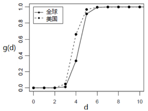
- g(d) 距离不超过d的连通的节点对的比例
- D 有效直径: g(D)=0.9
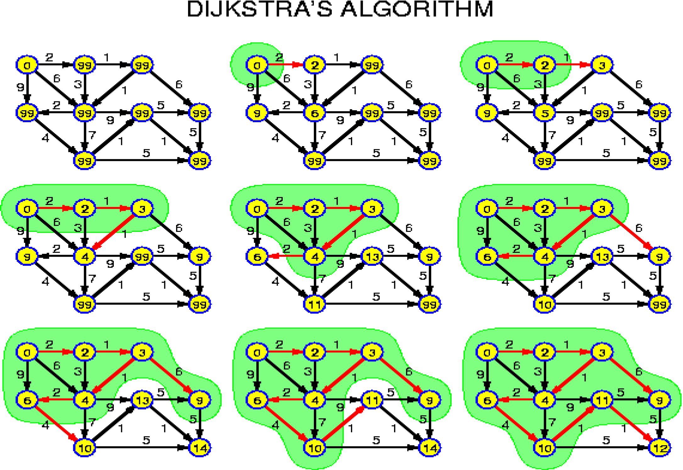
- 加权有向网络 (边数最少的路径并不一定是权值之和最小的路径)
- 经典算法:Dijkstra https://zhuanlan.zhihu.com/p/106269332
- Facebook任意两个用户之间距离不超过5的概率是92%
- 直径收缩 Shrinking diameters
import networkx as nx
import matplotlib.pyplot as plt

fig, ax1 = plt.subplots(figsize=(13, 4))#调整画布尺寸
plt.subplot(121)
nx.draw_networkx(G_kite)

print(G_kite[0])#获取邻居节点
print('0节点的邻节点为:',list(G_kite[0]))#将邻居节点装进一个列表中

#绘制0节点邻居形成的网络图
G_neibor0=nx.subgraph(G_kite,list(G_kite[0]))
plt.subplot(122)
nx.draw_networkx(G_neibor0,with_labels=True)
plt.show()

#获取邻节点网络的另一种方式
ego=nx.ego_graph(G_kite,0,center=False)#center参数表示是否加入中心节点,此处为0节点
nx.draw_networkx(ego,with_labels=True)
#计算风筝网络图0节点的聚类系数
print('风筝网络图中0节点的聚类系数:',round(nx.clustering(G_kite,0),3))
#计算0节点邻居形成的网络图密度
print('0节点邻居之间形成的网络图的密度:',round(nx.density(G_neibor0),3))

#计算0-9节点聚类系数
print('风筝网络图0-9节点的聚类系数依次为:',[round(i,3) for i in nx.clustering(G_kite).values()])

- 含义:节点聚类系数越高,意味着i的朋友之间互为朋友的平均概率越高
- 那$k_i=0$或$k_i=1$呢?($C_i=0$)
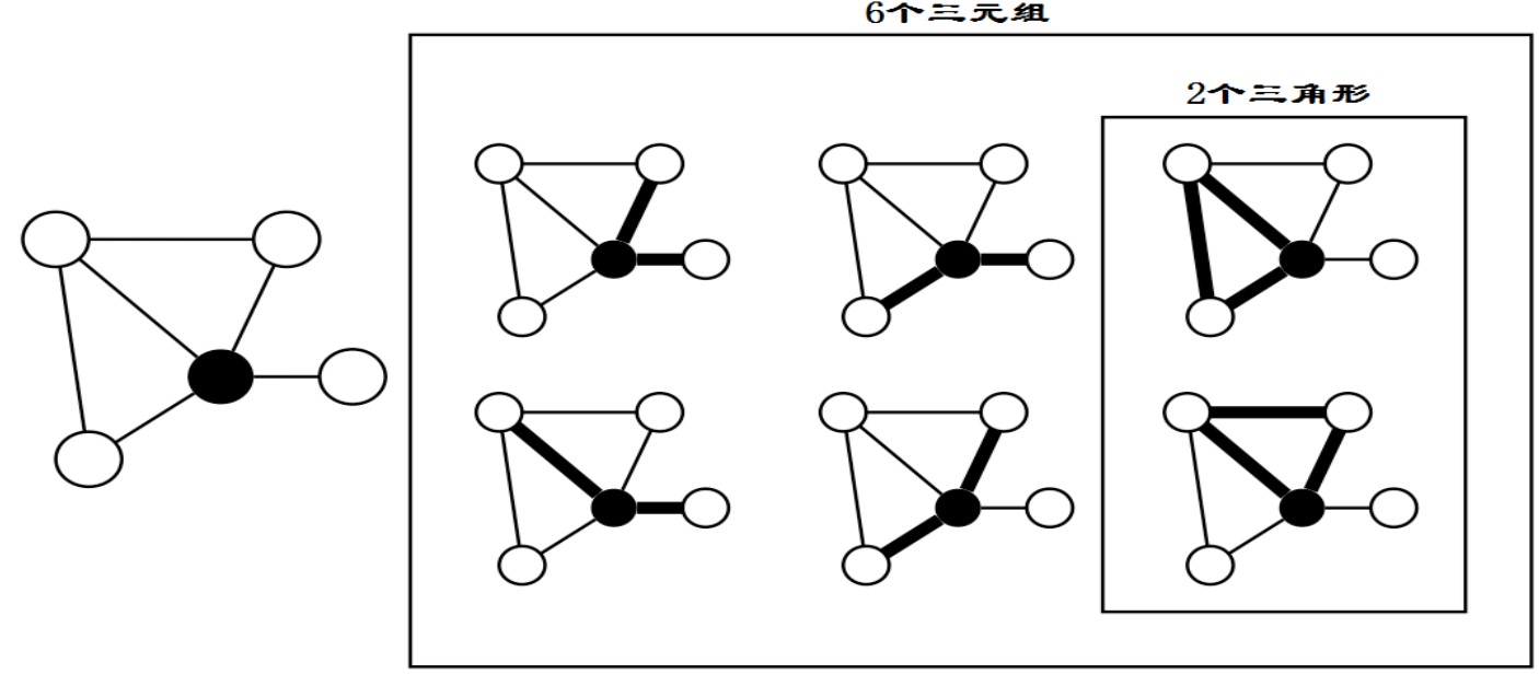
- 由此有另一个角度产生的定义:$C_i=\frac{包含节点i的三角形数目}{以节点i为中心的连通三元组的数目}$
- 每个包含节点i的三角形中有一边连接着i的两个邻节点,连通三元组保证节点i至少有两个邻节点
- 下图展示了两种连通三元组
4.2 网络聚类系数
- 定义1:网络中所有节点的聚类系数的平均值
- $C=\frac{1}{N}\sum_{i=1}^{N} {C_i}$
- 定义2:Transitivity 横截性,网络传递性
- $C=\frac{网络中三角形的数目}{网络中连通三元组的数目/3}$
- 边聚类系数、社团聚类系数
#计算图的平均聚类系数
print('风筝网络图的平均聚类系数:',round(nx.average_clustering(G_kite),3))
#计算图的横截性
print('风筝网络图的聚类系数:',round(nx.transitivity(G_kite),3))
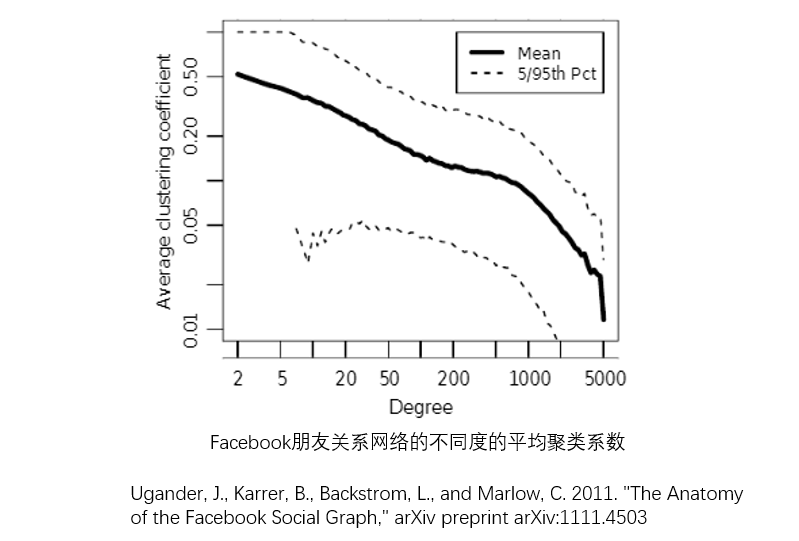
- 有时关注一类节点的整体行为或平均行为
- 度为k的节点的聚类系数的平均值
#计算平均度,方法1
import pandas as pd
import numpy as np
kite_D=pd.DataFrame(G_kite.degree())#获取各个节点的度
kite_D.columns=['node','degree']#重命名列名,默认为0,1
print('风筝网络图的平均度:',np.mean(kite_D['degree']))
print('\n')
#方法2:通过info函数直接获取
print(nx.info(G_kite))
5.2 平均度与密度
- 网络平均度与密度的关系:$\langle k\rangle=\frac{2M}{N}=(N-1)\rho \approx N\rho$
- $M(t)\sim N^\alpha(t)$
- 如果平均度是常数,那么网络就会越来越稀疏$\alpha=1$;如果密度是常数,那么平均度就会越来越大$\alpha=2$。
一般而言,介于二者之间$1<\alpha<2$。
大规模网络的一个通有特性是稀疏性:网络中实际存在的边数要远远小于最大可能的边数。
- 2011年5月,Facebook的朋友关系网络包含7.21亿活跃用户,687亿条边,网络平均度$\langle k\rangle=190$,密度为$\rho = 0.3\times10^{-7}$,是一个非常稀疏的网络。
- 随着时间的发展,平均度增加,但是网络也会越来越稀疏。
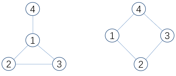
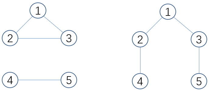
- 思考:以下两个网络图的平均度?
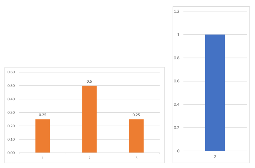
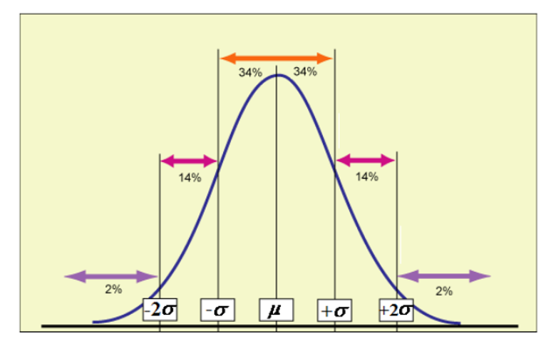
- 正态分布 Normal Distribution
- 最大值除以最小值一般是个有限的数值,绝大部分人居中
- $\xi\sim N(\mu,\sigma^2)$

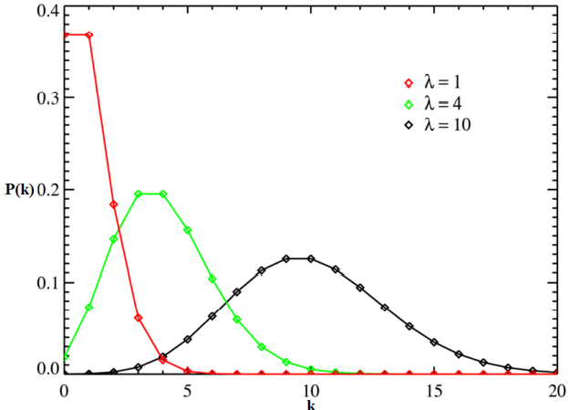
- 泊松分布 Poisson Distribution
- 泊松分布就是描述某段时间内,事件具体的发生概率。
- $P(k)=\frac{\lambda^ke^-\lambda}{k!}$
- 这里$\lambda$是这段时间内事件发生的平均次数;$k$是事件发生的次数。
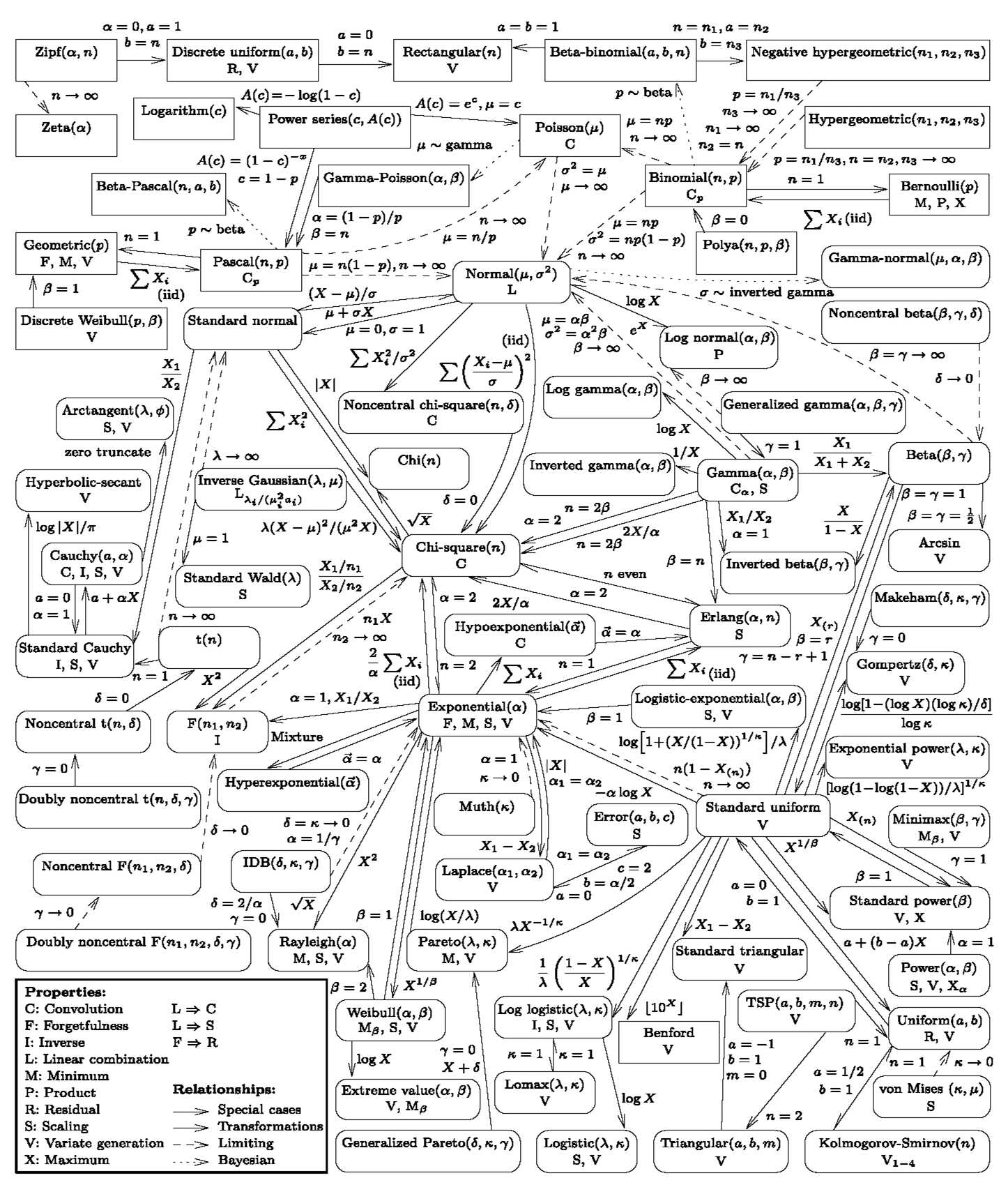
- 各种分布之间的关系
- 泊松分布是二项分布的极限,这是因为可以把这段时间切割成比较小的时间段,每个时间段扔硬币来决定事件是否发生(转成一个二项分布问题),而全部时段加起来事件发生的次数,既是二项分布的X,也是泊松分布的X。
- 因此,二项分布的$p$很小,而$N$又很大时,就会接近于泊松分布。
- 泊松分布的$\lambda$很大时,就会接近正态分布。
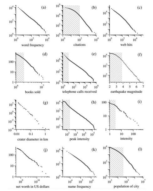
- 无标度分布、80/20法则、长尾分布
- 无标度分布:大部分节点度很小,少数节点度很大
- 80/20法则:管好少数节点,带动(忽略)多数节点
- 长尾分布:多数“小”节点的累积作用也不可忽视
幂律分布
- $P(k)\sim k^{-\gamma}$ ($\gamma>0$为幂指数,通常取值在2-3之间)
- 性质
- 无标度性质:一个概率分布函数$F(x)$,对于任意给定常数a存在常数b,使得$F(x)$满足$F(ax)=bF(x)$。
- 归一化
- 矩的性质
一个幂律分布的数据:数据
import pandas as pd
import matplotlib.pyplot as plt
# 读取边数据
powerlawdata=pd.read_csv('data//powerlawdata.csv')
powerlawdata.head()
plt.scatter(powerlawdata['msgcount'],powerlawdata['freq'],alpha=0.6)
plt.show()

plt.plot(powerlawdata['msgcount'],powerlawdata['freq'],alpha=0.6)
plt.show()

plt.loglog(powerlawdata['msgcount'],powerlawdata['freq'],alpha=0.6)
plt.show()

- 宇宙天体规模的幂律分布
- 地球 $1.276\times10^4km$ $5.965\times10^{24}kg$
- 太阳 $1.392\times10^6km$ $1.989\times10^{30}kg$
- 海山二 $240D\odot$ $120\sim200M\odot$
- 参宿四 $955D\odot$ $11.6M\odot$
- 大犬座 $1420M\odot$ $17M\odot$

- 生活中的幂律分布
5.4 财富分配
- 根据招行2019年报,1.84%的储户拥有81.2%的存款;而0.056%的储户拥有29.8%的存款。真实的财富分布可能更加极端,因为这只是存款,富有的人更有可能拥有其它资产;招行反映的只是城市群体,乡村的人更加贫穷。

美国的财富分布可视化分析。
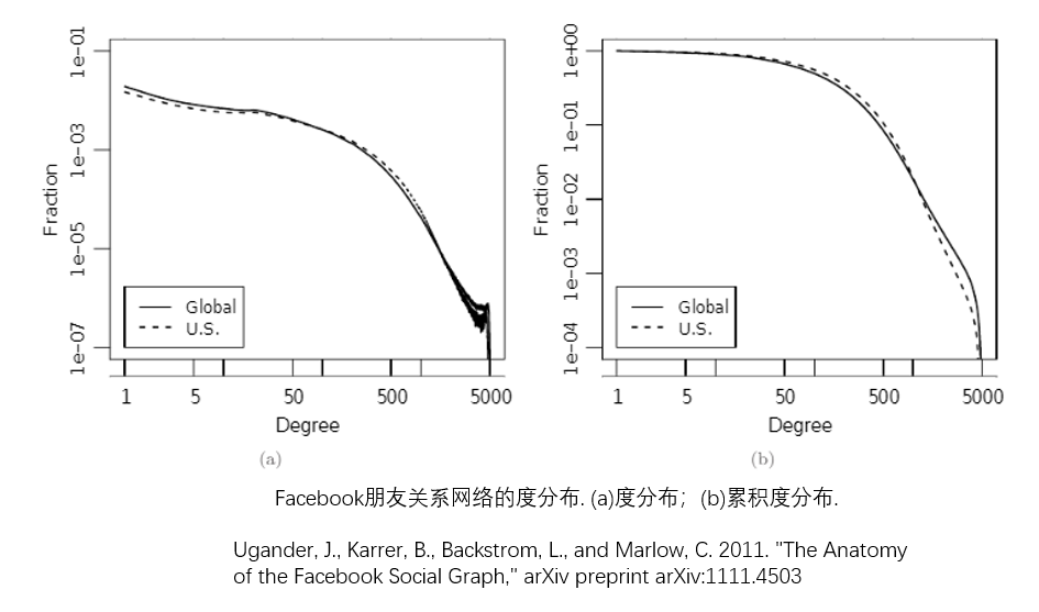
- 实际网络度分布
#绘制度分布图形的python代码
import pandas as pd
print('风筝网络图各节点的度:',G_kite.degree())
kite_D=pd.DataFrame(G_kite.degree())#将展示形式变为Dataframe
kite_D.columns=['node','degree']#重命名列名,默认为0,1
kite_D
G_club=nx.karate_club_graph()#Zachary的空手道俱乐部数据
import matplotlib.pyplot as plt
import pandas as pd
club_D=pd.DataFrame(G_club.degree())#将展示形式变为Dataframe
club_D.columns=['node','degree']#重命名列名,默认为0,1
fig, ax1 = plt.subplots(figsize=(13, 4))#调整画布尺寸
plt.subplot(121)
plt.hist(kite_D['degree'],density=True)
# 添加x轴和y轴标签
plt.xlabel('Degree')
plt.ylabel('Density')
plt.title('Degree distribution of G_kite')

plt.subplot(122)
plt.hist(club_D['degree'],density=True)
plt.xlabel('Degree')
plt.ylabel('Density')
plt.title('Degree distribution of G_club')
plt.show()# 显示图形

- 幂律分布的原因
- 马太效应,一种强者愈强、弱者愈弱的现象,广泛应用于社会心理学、教育、金融以及科学领域。
- 马太效应:圣经《新约·马太福音》里有一则寓言: 从前,一个国王要出门远行,临行前,交给3个仆人每人一锭银子,吩咐道:“你们去做生意,等我回来时,再来见我。”国王回来时,第一个仆人说:“主人,你交给我的一锭银子,我已赚了10锭。”于是,国王奖励他10座城邑。第二个仆人报告:“主人,你给我的一锭银子,我已赚了5锭。”于是,国王奖励他5座城邑。第三仆人报告说:“主人,你给我的1锭银子,我一直包在手帕里,怕丢失,一直没有拿出来。 ” 于是,国王命令将第三个仆人的1锭银子赏给第一个仆人,说:“凡是少的,就连他所有的,也要夺过来。凡是多的,还要给他,叫他多多益善。”。
- 1968年,美国科学史研究者罗伯特·莫顿(Robert K. Merton)提出这个术语用以概括一种社会心理现象:“相对于那些不知名的研究者,声名显赫的科学家通常得到更多的声望;即使他们的成就是相似的,同样地,在一个项目上,声誉通常给予那些已经出名的研究者”。
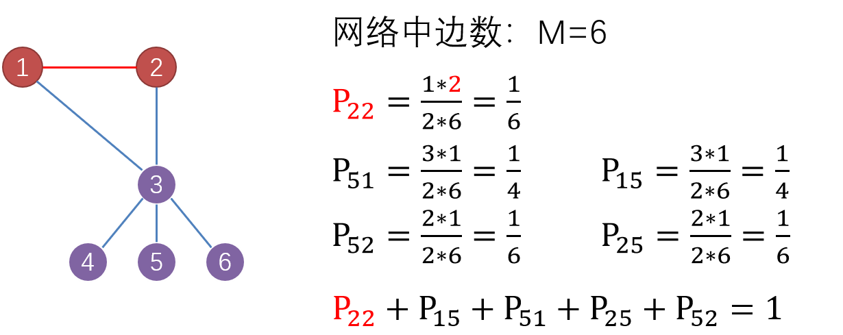
- 联合概率分布
- $P(j,k)$ 网络中随机选取的一条边的两个端点的度分别为$j$和$k$的概率
- 网络中度为$j$的节点和度为$k$的节点之间存在的边数占网络总边数的比例
- $P(j,k)=\frac{m(j,k)\mu(j,k)}{2M}$,其中,$m(j,k)$为度为$j$的节点和度为$k$的节点之间存在的边数,如果$j=k$,$\mu(j,k)=2$,否则$\mu(j,k)=1$
- 性质
- 对称性 $P(j,k)=P(k,j)$,对任意$j$, $k$
- 归一化 $\sum_{j,k=k_{min}}^{k_{max}} {P(j,k)}=1$
余度分布(excess degree distribution)
- 对于“余度”的理解:邻居的度。excess(超过的,遇到一个节点再往前多走一步,就是邻居的)degree
- 余度分布是“邻居的度分布”。余度这个词很诡异。
- $P_n(k)=\sum_{j=k_{min}}^{k_{max}} {P(j,k)}$
- 这里的$n$不是计数的$n$,应该是neighbour的 n
- 其中,$k_{min}$和$k_{max}$分别为网络中节点度最小值和最大值。$P_n(k)$为网络中随机选取的一个节点随机选取的一个邻居节点的度为$k$的概率
度为$k$的节点的余平均度 (excess average degree)
- 度为$k$的节点的邻居节点的平均度记为 $\langle k_{nn}\rangle(k)$
- 计算方法:
- 选出度为k的节点
- 计算每个度为k的节点的邻居节点的平均度(networkx中的average_neighbor_degree)
- 取平均
EAV_G=pd.DataFrame([nx.average_neighbor_degree(G_club)]).T
EAV_G1=EAV_G.reset_index().rename(columns={'index':'node',0:'AND'})#返回各个节点的余平均度(AND, Average Neighbour Degree)
Degree_G=pd.DataFrame(nx.degree(G_club))
Degree_G.columns=['node','degree']#返回各个节点的度
EAV_D=Degree_G.merge(EAV_G1)#进行组合,命名为EAV_D
#pd.concat([EAV_G1,Degree_G],axis=1)

print('各个节点的度和余平均度:')
print(EAV_D)

print('平均度为:',round(EAV_D['degree'].mean(),2),';  平均余度为:',round(EAV_D['AND'].mean(),2))

print('各个度的余平均度:')
print(round(EAV_D.groupby('degree')['AND'].mean(),3).reset_index(name='AND'))
好友悖论 Friendship Paradox
- 你的好友比你的好友多!
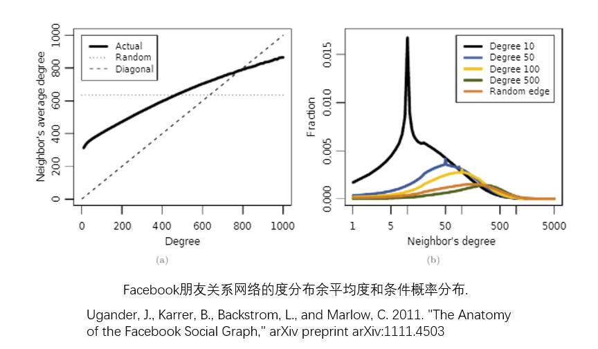
- 2011年5月,Johan Ugander、Brian Karrer、Lars Backstrom 、Cameron Marlow调查了Facebook上所有的活跃用户(当时为7.21亿人,约为世界人口的10%),其中共有690亿对好友关系。研究人员研究了用户们的数量与其朋友的朋友数量,发现93%的用户的朋友数量低于他朋友的朋友数量的平均值。之后,他们从整体上对Facebook进行了研究,发现平均一个用户有190个朋友,而他们的朋友平均有635个朋友。
- 余平均度与对角线交点在700左右,好友数超过700(仅8%),你的好友数大于你的好友的好友数;
- 因此,大部分人会发现,好友比自己更受欢迎。
- 原因:平均度只是简单平均,余平均度按照度做了加权平均,自然会更高(尝试证明?)
思考:如果换做是中位数、众数呢?
Scott Feld (1991). Why your friends have more friends than you do.
- Momeni, N., & Rabbat, M. (2016). Qualities and inequalities in online social networks through the lens of the generalized friendship paradox.Plos One, 11(2).
好友悖论的应用:受欢迎的人更容易被感染
- 尼古拉斯·克里斯塔基斯(Nicholas Christakis)是哈佛医学院一位从事医学和社会学跨界研究的教授。他和加州大学圣地亚哥分校医学院的一名教授詹姆斯·福勒(James Fowler)在科学杂志《PLoS One》上发表了一项研究成果,通过研究2009年流感对744名学生所产生的影响,他们找到了一种早期检测感染性疾病爆发的新方法。
- 克里斯塔基斯和他的同事们推断,处于社会网络中心的这些人会比边缘地带的人更早感染(流行性)疾病。这通过常识很容易理解:社交“花蝴蝶们”接触病源的可能性当然比普通人高。在2009年流感季节临近时,克里斯塔基斯和费得设计了一个实验,验证他们的推断。他们联系了319名哈佛大学的学生,让他们列举出425名朋友,以这425个人作为“朋友组”,与另一个“随机组”做对照,通过自报症状和哈佛大学健康服务中心提供的数据进行对比、检测。
- 结果在他们意料之中。“朋友组”和“随机组”相比,提早两周出现了流感症状。而通过另一种检测方法,克里斯塔基斯甚至观察到“朋友组”疫情流行出现高峰期的时间,比“随机组”早了整整46天。克里斯塔基斯认为这对公共卫生而言可能具有重要意义。“通过简单地询问一个随机人群,让其列举自己朋友的名字,然后追踪并比较两组人群,我们就能够在疫情攻击社会整体人口前预测出疫情的走向,从而允许相关政府部门采取一种更早、更有力,也更有效的措施。”他说。
- 尼古拉斯·克里斯塔基斯(Nicholas Christakis)发表的文章
- Christakis, NA; Allison, PD (2006). “Mortality after the Hospitalization of a Spouse” (PDF). New England Journal of Medicine. 354 (7): 719–730.
- Christakis, NA; Fowler, JH (2007). “The Spread of Obesity in a Large Social Network Over 32 Years” (PDF). New England Journal of Medicine. 357 (4): 370–379.
- Elwert, F; Christakis, NA (2008). “The Effect of Widowhood on Mortality by the Causes of Death of Both Spouses” (PDF). American Journal of Public Health. 98 (11): 2092–2098.
- Christakis, NA; Fowler, JH (2008). “Quitting in Droves: Collective Dynamics of Smoking Behavior in a Large Social Network” (PDF). New England Journal of Medicine. 358 (21): 2249–2258.
- Fowler, JH; Christakis, NA (2009). “The Dynamic Spread of Happiness in a Large Social Network” (PDF). British Medical Journal. 337 (768): a2338.
- Fowler, JH; Dawes, CT; Christakis, NA (2009). “Model of genetic variation in human social networks”. Proceedings of the National Academy of Sciences. 106 (6): 1720–1724.
- Fowler, JH; Christakis, NA (2010). “Cooperative Behavior Cascades in Human Social Networks”. Proceedings of the National Academy of Sciences. 107 (12): 5334–8.
- Christakis, NA; Fowler, JH (2010). “Social Network Sensors for Early Detection of Contagious Outbreaks”. PLOS ONE. 5 (9): e12948.
- Fowler, JH; Settle, JE; Christakis, NA (2011). “Correlated Genotypes in Friendship Networks”. Proceedings of the National Academy of Sciences. 108 (5): 1993–7.
- Rand, DG; Arbesman, S; Christakis, NA (2011). “Dynamic Social Networks Promote Cooperation in Experiments with Humans”. Proceedings of the National Academy of Sciences. 108 (48): 19193–8.
- Apicella, CL; Marlowe, FW; Fowler, JH; Christakis, NA (2012). “Social Networks and Cooperation in Hunter-Gatherers” (PDF). Nature. 481 (7382): 497–501.
- Christakis, NA; Fowler, JH (2014). “Friendship and Natural Selection”. Proceedings of the National Academy of Sciences. 111 (3): 10796–10801.
- Nishi, CL; Shirado, FW; Rand, DG; Christakis, NA (2015). “Inequality and Visibility of Wealth in Experimental Social Networks”. Nature. 526 (7382): 426–429.
- Kim, DA; Hwong, AR; Stafford, D; Hughes, DA; O’Malley, AJ; Fowler, JH; Christakis, NA (2015). “Social Network Targeting to Maximize Population Behavior Change: A Cluster Randomised Controlled Trial”. The Lancet. 386 (9989): 145–153.
- Shirado, H; Christakis, NA (2017). “Locally Noisy Autonomous Agents Improve Global Human Coordination in Network Experiments”. Nature. 545 (7654): 370–374.
- Traeger, ML; Sebo, SS; Jung, M; Scassellati, B; Christakis, NA (2020). “Vulnerable Robots Shape Human Conversational Dynamics in a Human-Robot Team”. Proceedings of the National Academy of Sciences. 117 (12): 6370–6375.
- Jia, JS; Lu, X; Yuan, Y; Xu, G; Jia, J; Christakis, NA (2020). “Population Flow Drives Spatio-Temporal Distribution of COVID-19 in China”. Nature. 582 (7812): 389–394.
- Shirado, H; Christakis, NA (2020). “Network Engineering Using Autonomous Agents Increases Cooperation in Human Groups”. iScience. 23 (9): 101438.
- Alexander, M; Forastiere, L; Gupta, S; Christakis, NA. (2022-07-26). “Algorithms for seeding social networks can enhance the adoption of a public health intervention in urban India”. Proceedings of the National Academy of Sciences. 119 (30): e2120742119.
6.2 度相关性
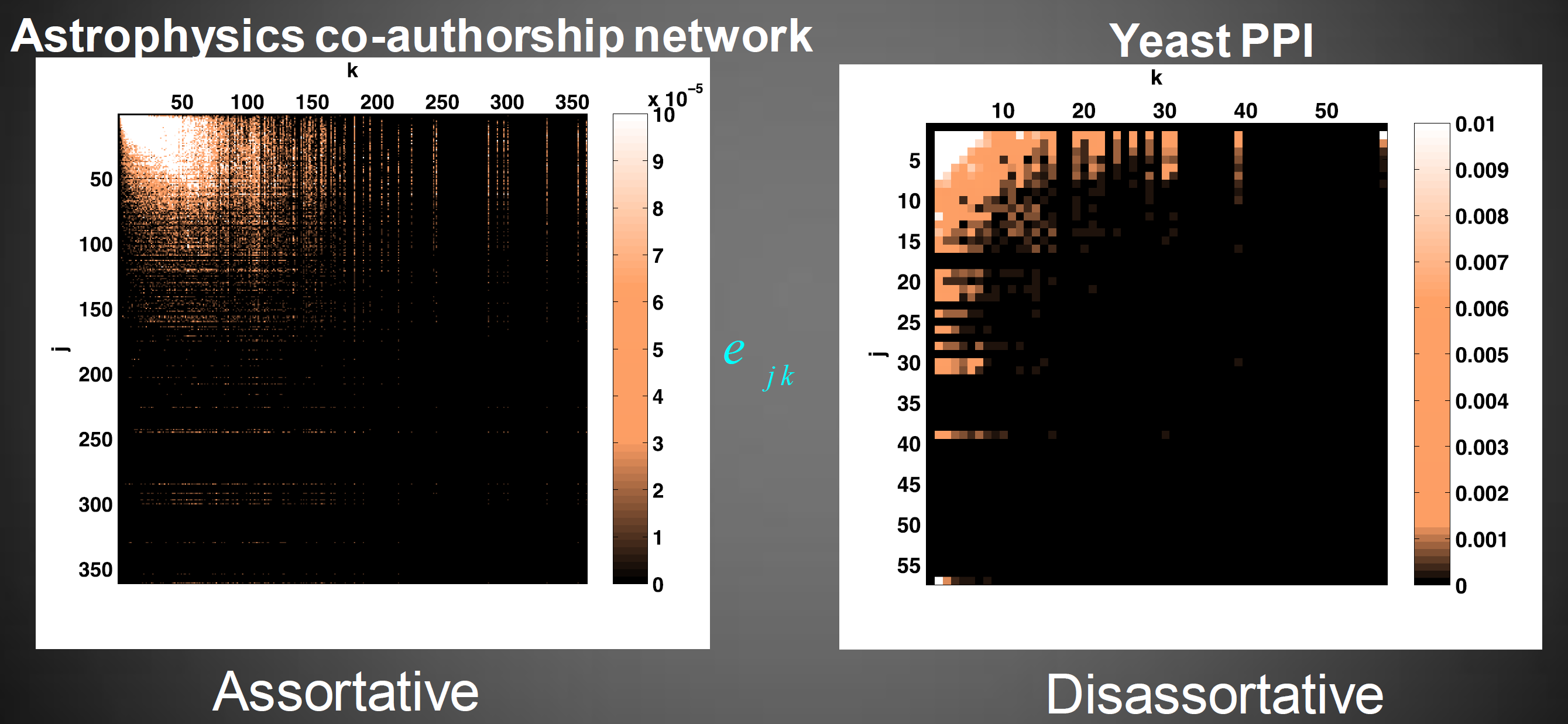
$e_{jk}$ 网络中随机选取的一条边的两个端点的度分别为$j$和$k$的概率。(就是前面讲的 $P(j,k)$)
- $\sum_{{j,k}}{e_{jk}}=1$
$q_k$ 网络中随机选取的一条边的端点的度为$k$的概率。(就是前面讲的 $P(k)$)
- $\sum_{j}{e_{jk}}=q_k$
$e_{jk}=q_jq_k\ \forall j,k$,则网络不具有相关性,否则具有相关性。(就是 $P(j,k)=P(j)P(k)$)
对$e_{jk}$可视化
print('各边节点度情况',list(nx.node_degree_xy(G_club))) #对于无向图每个边会计算两次,因为没有指定的方向(nx.node_degree_xy(G_kite)))
nx.draw_networkx(G_club,with_labels=True)

# 统计每一种节点度的组合在所有边中占的比例
G_edge=pd.DataFrame(nx.node_degree_xy(G_club))
G_edge.columns=['degree_of_node1','degree_of_node2']
G_degree=G_edge.groupby(by=['degree_of_node1','degree_of_node2']).size().reset_index(name='count')
G_degree['percentage']=round(G_degree['count']/G_degree['count'].sum(),3)
G_degree
pt = G_degree.pivot_table(index='degree_of_node1', columns='degree_of_node2', values='percentage')
import seaborn as sns
sns.set_context({"figure.figsize":(8,8)})
sns.heatmap(data=pt,cmap="RdBu_r")#色带YlGnBu
#相关性不是很明显,节点太少

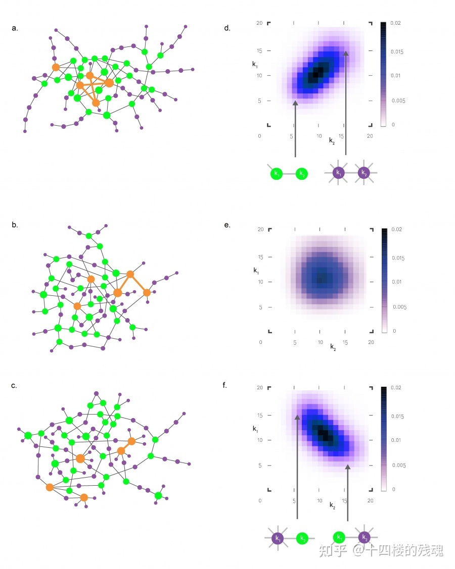
同配系数 assortativity coefficient
- 使用$e_{jk}$和$q_k$差值来刻画
- $\langle jk\rangle-\langle j\rangle\langle k\rangle=\sum_{j,k}{jk(e_{jk}-q_jq_k)}$
- 归一化处理(利用余度分布的方差)
- 归一化的相关系数,称为同配系数(assortativity coefficient)
- $r=\frac{1}{\sigma_q^2}\sum_{j,k}{jk(e_{jk}-q_jq_k)}$,其中 $\sigma_q=\sum_k{k^2{q_k}^2}-[\sum_k{k{q_k}}]^2$
- 同配系数$r>0$表示整个网络呈现同配性结构,度大的节点倾向于和度大的节点相连;$r<0$表示整个网络呈现异配性;$r=0$表示网络结构不存在相关性
- 社交网络是同配还是异配?
- 思考:富人俱乐部与同配系数的关系。
print('度相关系数:',round(nx.degree_pearson_correlation_coefficient(G_club),3))
print('度同配系数:',round(nx.degree_assortativity_coefficient(G_club),3)) #归一化的相关系数
#两者等价
fig, ax1 = plt.subplots(figsize=(13, 4))#调整画布尺寸
plt.subplot(121)
G1 = nx.Graph()
G1.add_nodes_from([0, 1], color="red")
G1.add_nodes_from([2, 3,4], color="blue")
G1.add_edges_from([(0, 1), (2, 3),(3,4)])
node_color1=[G1.nodes[v]['color'] for v in G1]#获得G1中各个节点的设置值
nx.draw_networkx(G1,with_labels=True, node_color=node_color1)

plt.subplot(122)
G2 = nx.Graph()
G2.add_nodes_from([1, 3], color="red")
G2.add_nodes_from([0, 2,4], color="blue")
G2.add_edges_from([(0, 1), (2, 3),(1,4)])
node_color2=[G2.nodes[v]['color'] for v in G2]#获得G2中各个节点的设置值
nx.draw_networkx(G2,with_labels=True, node_color=node_color2)

print('第一张图属性同配系数:',round(nx.attribute_assortativity_coefficient(G1, "color"),3))
print('第二张图属性同配系数:',round(nx.attribute_assortativity_coefficient(G2, "color"),3))
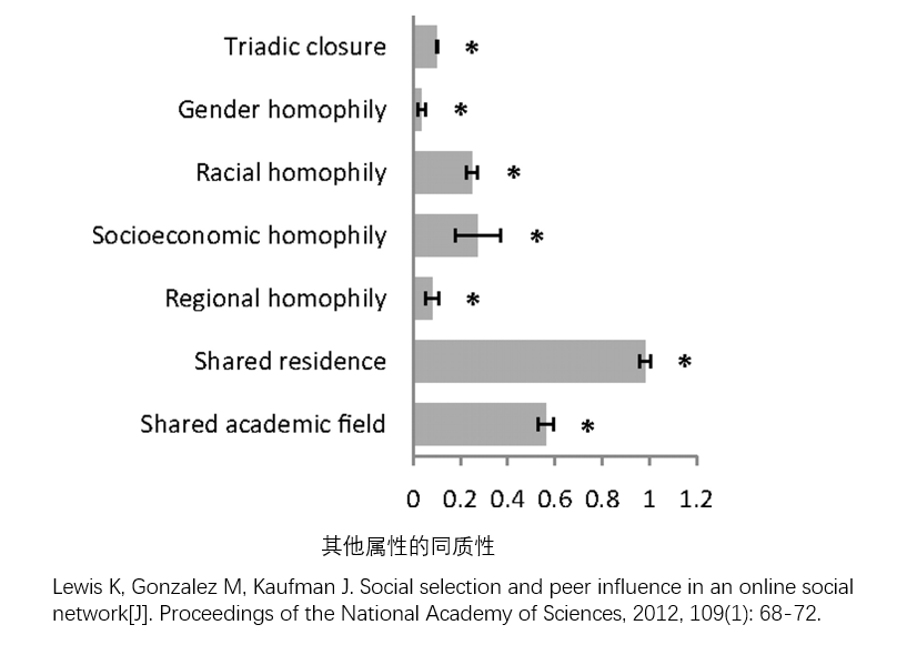
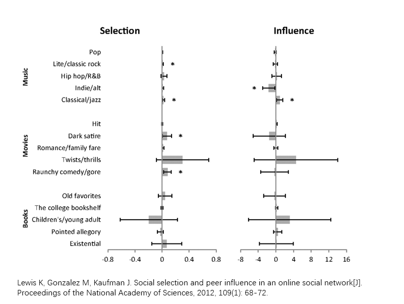
- 关于同质性的解释:
- 选择(Selection):人们倾向于和相似的人成为朋友
- 影响(Influence):近朱者赤,近墨者黑
- 如何区分选择和影响这两个因素? 如何判断哪一个因素起着更大的作用?
- 需要关于社会关系和个体属性的详细的随时间演化的数据;以及对结构和个体行为的联合演化建立合适的模型
- 我们的工作:
- 冉晓斌,刘跃文*,姜锦虎,(2017). 数据驱动下的个体移动服务产品采纳行为的扩散研究,中国管理科学,2017 Vol. 25 (9): 141-147. Download
Homework
- 利用课堂上提供的一个社交网络数据,计算网络指标并进行评估
- 探究该社交网络是同配还是异配。
- 尝试证明好友悖论。